\[\require{mhchem}\]

Deprotonation Reactions

In many applications, it is crucial to know the protonation state of a molecule. For example, in ion exchange chromatography only charged molecules can adsorb on the resin, i.e. positively charged ions on a cation exchanger, or negatively charged ions on an anion exchanger. However, the charge of the molecule is a function of the pH value of the solution. For this purpose, the pH, which is often also influenced by other acids or bases, has to be considered when modelling the system.

Since the \(pH\) is defined as:

\[ pH = -log_{10}(\ce{[H^+]}), \]

it can be derived from knowing the proton concentration, which in turn is a result of reaction equilibria of the protonation and deprotonation reactions. There reactions are characterized by their \(pK_a\) value:

\[ \ce{A <=>[K_{a}] A^{-} + H^{+}} \]

\[ K_{a} = \frac{\ce{[A^{-}]}\ce{[H^{+}]}}{\ce{[HA]}} \]

\[ pK_{a} = -log_{10}(K_{a}) \]

To model the \(pH\) in CADET, the different protonation states of molecules can be treated as individual (pseudo-) components which are coupled via chemical reactions. Currently, reactions in rapid equilibrium are not implemented in CADET but can be approximated by scaling up the reaction rate.

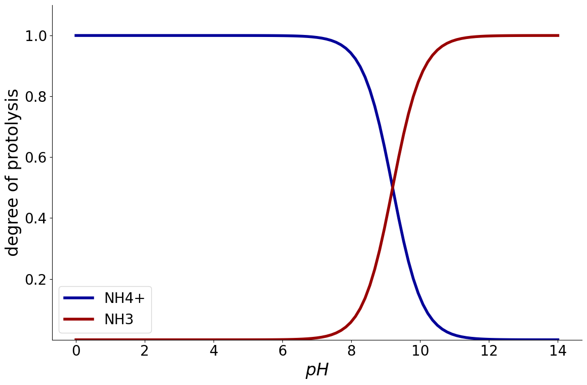
Example: Ammonia

Ammonia is a base and can thusly accept protons:

\[ \ce{NH3 + H^{+} <=>[pK_{a}] NH4^{+}}. \]

With a \(pK_{a}\) value of 9.2, it is mostly positively charged for pH values lower than 9.2

from CADETProcess.processModel import ComponentSystem

component_system = ComponentSystem()

component_system.add_component(
	'H+',
	charge=1
)
component_system.add_component(
	'Ammonia',
	species=['NH4+', 'NH3'],
	charge=[1, 0]
)

Then, the CADETProcess.processModel.MassActionLaw reaction model is defined. The CADETProcess.processModel.MassActionLaw.add_reaction() method expects the following arguments:

• component indices

• stoichiometric coefficients

• forward reaction rate

• backward reaction rate (or, if the reaction is considered quasi-stationary, is_kinetic=False)

If the acid undergoes more than one dissociation reaction, the reactions need to be added with increasing \(pK_a\) values. For more information about configuring reaction models, refer to Chemical Reactions.

from CADETProcess.processModel import MassActionLaw
reaction_system = MassActionLaw(component_system)

reaction_system.add_reaction(
	[1, 2, 0], [-1, 1, 1], 10**(-9.2)*1e3, is_kinetic=False
)

The reaction can now be associated with any unit operation model CADET-Process.

CADET-Process also provides functionality to determine the charged species as a function of \(pH\). For this purpose, the CADETProcess.equilibria module needs to be imported and the reaction system, as well as the \(pH\) need to be passed to the CADETProcess.equilibria.charge_distribution() function.

from CADETProcess import equilibria

pH = 7
print(equilibria.charge_distribution(reaction_system, pH))

[0.99372999 0.00627001]

Since \(\ce{NH4^+}\) is the first component, this shows that at \(pH = 7\), most of the ammonia is positively charged.

The CADETProcess.equilibria module also provides a function to plot the charge distribution as a function of \(pH\). For this purpose, pass the previously configured reaction model to the CADETProcess.equilibria.plot_charge_distribution() function.

from CADETProcess import equilibria
_ = equilibria.plot_charge_distribution(reaction_system)

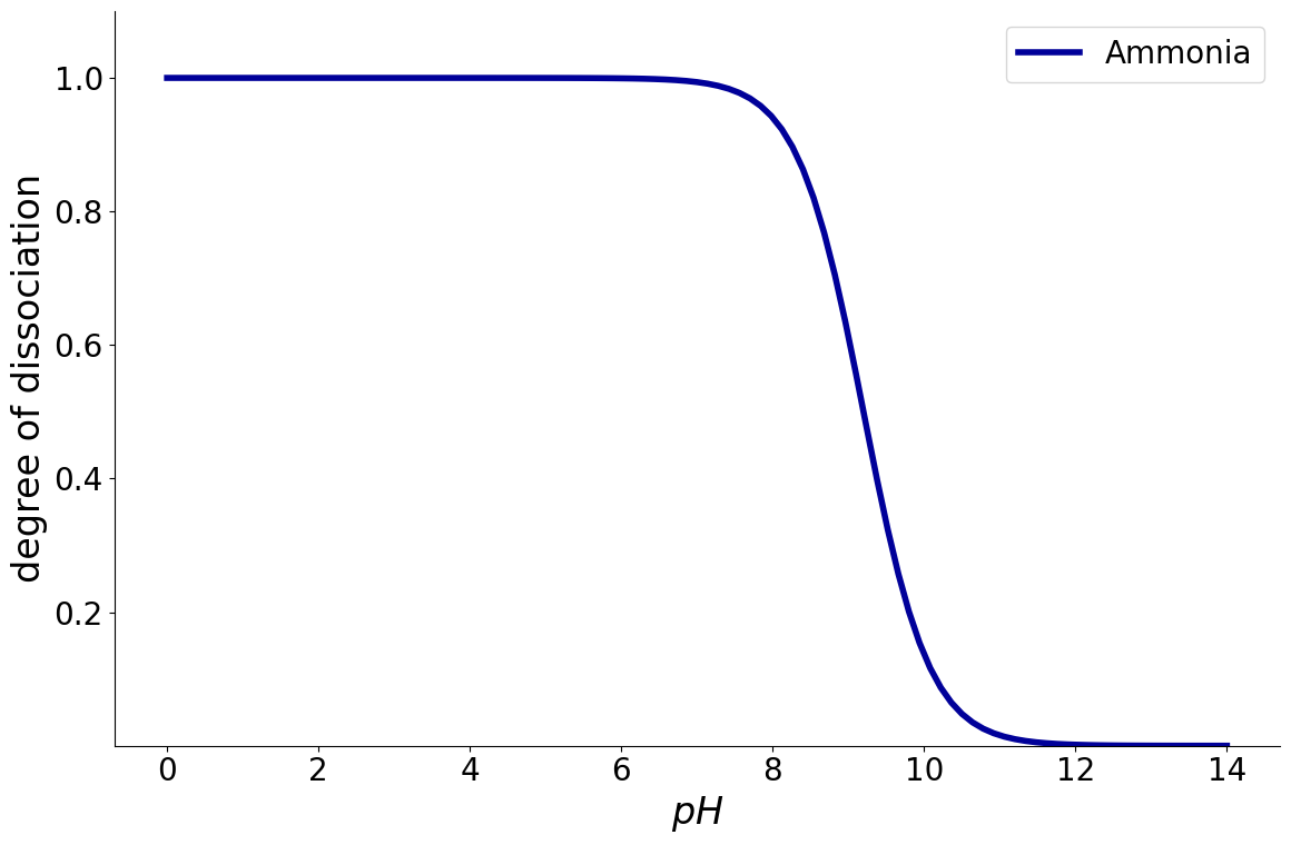
Optionally, also cumulative charge distribution can be plotted which adds up all the individual components:

_ = equilibria.plot_charge_distribution(reaction_system, plot_cumulative=True)

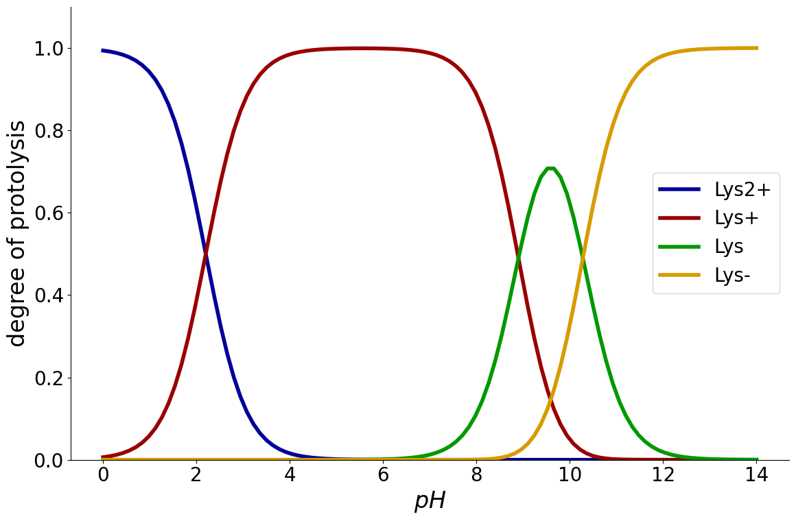
Example: Lysine

Because all amino acids contain amine and carboxylic acid functional groups, they are amphiprotic. This means, they can either donate or accept a proton and hence react both as an acid and as a base.

For this purpose, the protonation and deprotonation of amino acids is modelled as multiple chemical reactions. In case of Lysine, three reactions are required to model the behaviour

\[\begin{split} \ce{Lys^{2+} <=>[pK_{a,1}] Lys^{+} + H^{+}}\\ \ce{Lys^{+} <=>[pK_{a,2}] Lys^{} + H^{+}}\\ \ce{Lys^{} <=>[pK_{a,3}] Lys^{-} + H^{+}}, \end{split}\]

using the following \(pK_a\) values:

\[\begin{split} pK_{a,1} = 2.20\\ pK_{a,2} = 8.90\\ pK_{a,3} = 10.28. \end{split}\]

component_system = ComponentSystem()
component_system.add_component(
    'H+',
    charge=1
)
component_system.add_component(
    'Lysine',
    species=['Lys2+', 'Lys+', 'Lys', 'Lys-'],
    charge=[2, 1, 0, -1]
)

reaction_system = MassActionLaw(component_system, name='Lysine')
reaction_system.add_reaction(
    [1, 2, 0], [-1, 1, 1], 10**(-2.20)*1e3, is_kinetic=False
)
reaction_system.add_reaction(
    [2, 3, 0], [-1, 1, 1], 10**(-8.90)*1e3, is_kinetic=False
)
reaction_system.add_reaction(
    [3, 4, 0], [-1, 1, 1], 10**(-10.28)*1e3, is_kinetic=False
)

Again, the charge distribution can be plotted:

_ = equilibria.plot_charge_distribution(reaction_system)
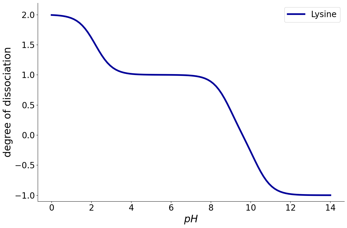
_ = equilibria.plot_charge_distribution(reaction_system, plot_cumulative=True)