Optimization Problem#

The OptimizationProblem class is used to specify optimization variables, objectives and constraints. To instantiate a OptimizationProblem, a name needs to be passed as argument.

from CADETProcess.optimization import OptimizationProblem

optimization_problem = OptimizationProblem('single_objective')

By default, the OptimizationProblem uses a DiskCache to store intermediate evaluation results. In contrast to using a simple python dictionary, this also allows for multi-core parallelization.

Optimization Variables#

Any number of variables can be added to the OptimizationProblem. To add a variable, use the add_variable() method. The first argument is the name of the variable. Optionally, lower and upper bounds can be specified.

optimization_problem.add_variable('var_0', lb=0, ub=100)

OptimizationVariable(name=var_0, evaluation_objects=[], parameter_path=None, lb=0, ub=100)

Note that for many situations, it can be advantageous to normalize the optimization variables to ensure that all parameters are on a similar scale. For more information, refer to Variable Normalization.

The total number of variables is stored in n_variables and the names in variable_names.

print(optimization_problem.n_variables)
print(optimization_problem.variable_names)

1
['var_0']

In order to reduce the complexity of the optimization problem, dependencies between individual variables can be defined. For more information, refer to Variable Dependencies.

For more information on how to configure optimization variables of multi-dimensional parameters, refer to {ref}`variable_indices_gude.

Objectives#

Any callable function that takes an input \(x\) and returns objectives \(f\) can be added to the OptimizationProblem. Consider a quadratic function which expects a single input and returns a single output:

def objective(x):
	return x**2

To add this function as objective, use the add_objective() method.

optimization_problem.add_objective(objective)

It is also possible to use CADET-Process for multi-objective optimization problems. Consider the following function which takes two inputs and returns two outputs.

\[ f(x,y) = [x^2 + y^2, (x-2)^2 + (y-2)^2] \]

Either two callables are added as objective

import numpy as np

def objective_1(x):
	return x[0]**2 + x[1]**2

optimization_problem.add_objective(objective_1)

def objective_2(x):
	return (x[0] - 2)**2 + (x[1] - 2)**2

optimization_problem.add_objective(objective_2)

Alternatively, a single function that returns both objectives can be added. In this case, the number of objectives the function returns needs to be specified by adding n_objectives as argument.

def multi_objective(x):
	f_1 = x[0]**2 + x[1]**2
	f_2 = (x[0] - 2)**2 + (x[1] - 2)**2
	return np.hstack((f_1, f_2))

optimization_problem.add_objective(multi_objective, n_objectives=2)

In both cases, the total number of objectives is stored in n_objectives.

optimization_problem.n_objectives

For more information on multi-objective optimization, also refer to Multi-Objective Optimization.

The objective(s) can be evaluated with the evaluate_objectives() method.

optimization_problem.evaluate_objectives([1, 1])

array([2., 2.])

It is also possible to evaluate multiple sets of input variables at once by passing a 2D array to the evaluate_objectives_population() method.

optimization_problem.evaluate_objectives_population([[0, 1], [1, 1], [2, -1]])

array([[1., 5.],
       [2., 2.],
       [5., 9.]])

For more complicated scenarios that require (multiple) preprocessing steps, refer to Evaluation Toolchains.

Linear constraints#

Linear constraints are a common way to restrict the feasible region of an optimization problem. They are typically defined using linear functions of the optimization:

\[ A \cdot x \leq b, \]

where \(A\) is an \(m \times n\) coefficient matrix and \(b\) is an \(m\)-dimensional vector and \(m\) denotes the number of constraints, and \(n\) the number of variables, respectively.

In CADET-Process, each row \(a\) of the constraint matrix needs to be added individually. The add_linear_constraint() function takes the variables subject to the constraint as first argument. The left-hand side \(a\) and the bound \(b_a\) are passed as second and third argument. It is important to note that the column order in \(a\) is inferred from the order in which the optimization variables are passed.

For example, consider the following linear inequalities as constraints:

\[\begin{split} x_1 + x_3 ≤ 4, \\ 2x_2 – x_3 ≥ –2, \\ x_1 – x_2 + x_3 – x_4 ≥ 9. \end{split}\]

optimization_problem.add_linear_constraint(['var_1', 'var_3'], [1, 1], 4)
optimization_problem.add_linear_constraint(['var_2', 'var_3'], [-2, 1], 2)
optimization_problem.add_linear_constraint(['var_1', 'var_2', 'var_3', 'var_4'], [-1, 1, -1, 1], -9)

The combined coefficient matrix \(A\) is stored in the attribute A, and the right-hand side vector \(b\) in b. To evaluate linear constraints, use evaluate_linear_constraints().

optimization_problem.evaluate_linear_constraints([0, 0, 0, 0])

array([-4., -2.,  9.])

Any value larger than \(0\) means the constraint is not met. Alternatively, use check_linear_constraints() which returns True if all constraints are met (False otherwise).

optimization_problem.check_linear_constraints([0, 0, 0, 0])

False

Nonlinear constraints#

In addition to linear constraints, nonlinear constraints can be added to the optimization problem. To add nonlinear constraints, use the add_nonlinear_constraint() method.

Consider this function which returns the product of all input values.

def nonlincon(x):
    return np.prod(x)

To add this function as nonlinear constraint, use the add_nonlinear_constraint() method.

optimization_problem.add_nonlinear_constraint(nonlincon)

As with objectives, it is also possible to add multiple nonlinear constraint functions or a function that returns more than a single value. For the latter case, add n_nonlinear_constraints to the method.

To evaluate the nonlinear constraints, use evaluate_nonlinear_constraints().

optimization_problem.evaluate_nonlinear_constraints([0.5, 0.5])

array([0.25])

Alternatively, use check_nonlinear_constraints() which returns True if all constraints are met (False otherwise).

optimization_problem.check_nonlinear_constraints([0.5, 0.5])

False

By default, any value larger than \(0\) means the constraint is not met. If other bounds are required, they can be specified when registering the function. For example if the product must be smaller than 1, set bounds=1 when adding the constraint.

optimization_problem.add_nonlinear_constraint(nonlincon, bounds=1)

Note that evaluate_nonlinear_constraints() still returns the same value.

optimization_problem.evaluate_nonlinear_constraints([0.5, 0.5])

array([0.25])

To only compute the constraint violation, use evaluate_nonlinear_constraints_violation().

optimization_problem.evaluate_nonlinear_constraints_violation([0.5, 0.5])

array([-0.75])

In this context, a negative value denotes that the constraint is met.

The check_nonlinear_constraints() method also takes bounds into account.

optimization_problem.check_nonlinear_constraints([0.5, 0.5])

True

For more complicated scenarios that require (multiple) preprocessing steps, refer to Evaluation Toolchains.

Initial Values#

Initial values in optimization refer to the starting values of the decision variables for the optimization algorithm. These values are typically set by the user and serve as a starting point for the optimization algorithm to begin its search for the optimal solution. The choice of initial values can have a significant impact on the success of the optimization, as a poor choice may lead to the algorithm converging to a suboptimal solution or failing to converge at all. In general, good initial values should be as close as possible to the true optimal values, and should take into account any known constraints or bounds on the decision variables.

To facilitate the definition of starting points, the OptimizationProblem provides the create_initial_values().

Note

This method only works if all optimization variables have defined lower and upper bounds.

Moreover, this method only guarantees that linear constraints are fulfilled. Any nonlinear constraints may not be satisfied by the generated samples, and nonlinear parameter dependencies can be challenging to incorporate.

By default, the method returns a random point from the feasible region of the parameter space.

optimization_problem.create_initial_values()

array([[ 0.4581154 , -5.28133487]])

Alternatively, the Chebyshev center of the polytope can be computed, which is the center of the largest Euclidean ball that is fully contained within that polytope.

optimization_problem.get_chebyshev_center()

array([ 3.33333333, -3.33333333])

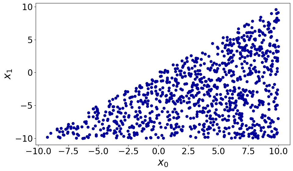
It is also possible to generate multiple samples at once. For this purpose, hopsy is used to efficiently (uniformly) sample the parameter space.

x = optimization_problem.create_initial_values(n_samples=1000)

import matplotlib.pyplot as plt
fig, ax = plt.subplots()
ax.scatter(x[:, 0], x[:, 1])
ax.set_xlabel(r'$x_0$')
ax.set_ylabel(r'$x_1$')
fig.tight_layout()

../../_images/388adbddd1df9bd1092ea740d5e56fc108d85d1b9dc736f464744eef4ad5f2cb.png

Callbacks#

A callback function is a user defined function that is called periodically by the optimizer in order to allow the user to query the state of the optimization. For example, a simple user callback function might be used to plot results.

All callback functions will be called with the best individual or with every member of the Pareto front in case of multi-objective optimization. For more information on controlling the members of the Pareto front, refer to Multi-criteria decision making (MCDM).

The callback signature may include any of the following arguments:

results : obj x or final result of evaluation toolchain.
individual : Individual, optional Information about current step of optimzer.
evaluation_object : obj, optional Current evaluation object.
callbacks_dir : Path, optional Path to store results.

Introspection is used to determine which of the signatures above to invoke.

def callback(results, individual, evaluation_object, callbacks_dir):
    print(results)
    print(individual.x, individual.f)
    print(evaluation_object)
    print(callbacks_dir)

For more information about evaluation toolchains, refer to Evaluation Toolchains.

To add the function to the OptimizationProblem, use the add_callback() method.

optimization_problem.add_callback(callback)

By default, the callback is called after every iteration/generation. To change the frequency, add a frequency argument which denotes the number of iterations/generations after which the callback function(s) is/are evaluated.