Closed Loop Recycling Process#

In closed-loop recycling (CLR), the stock mixture is pumped over the column several times until the desired purity is achieved. The general structure of a CLR is shown below.

../../_images/clr_flow_sheet.svg — Flow sheet for closed-loop recycling process.#

To realize the recycling, the output_state of the column needs to be modified, leading to the following event structure:

../../_images/clr_events.svg — Events for closed-loop recycling process.#

For this example, consider a two-component system with a Langmuir isotherm.

Component System#

from CADETProcess.processModel import ComponentSystem

component_system = ComponentSystem(['A', 'B'])

Binding Model#

from CADETProcess.processModel import Langmuir

binding_model = Langmuir(component_system, name='langmuir')
binding_model.adsorption_rate = [0.04, 0.05]
binding_model.desorption_rate = [1, 1]
binding_model.capacity = [100, 100]

Unit Operations#

from CADETProcess.processModel import (
    Inlet, Cstr, LumpedRateModelWithoutPores, Outlet
)
feed = Inlet(component_system, name='feed')
feed.c = [10, 10]

eluent = Inlet(component_system, name='eluent')
eluent.c = [0, 0]

pump = Cstr(component_system, name='pump')
pump.V = 1e-9

column = LumpedRateModelWithoutPores(component_system, name='column')
column.binding_model = binding_model
column.length = 0.6
column.diameter = 0.024
column.axial_dispersion = 4.7e-7
column.total_porosity = 0.7

outlet = Outlet(component_system, name='outlet')

Flow Sheet#

from CADETProcess.processModel import FlowSheet

flow_sheet = FlowSheet(component_system)

flow_sheet.add_unit(feed, feed_inlet=True)
flow_sheet.add_unit(eluent, eluent_inlet=True)
flow_sheet.add_unit(pump)
flow_sheet.add_unit(column)
flow_sheet.add_unit(outlet, product_outlet=True)

flow_sheet.add_connection(feed, column)
flow_sheet.add_connection(eluent, column)
flow_sheet.add_connection(column, outlet)
flow_sheet.add_connection(column, pump)
flow_sheet.add_connection(pump, column)

Process#

from CADETProcess.processModel import Process
process = Process(flow_sheet, 'clr')

Create Events and Durations#

Q = 60/(60*1e6)

process.add_event('feed_on', 'flow_sheet.feed.flow_rate', Q)
process.add_event('feed_off', 'flow_sheet.feed.flow_rate', 0.0)

process.add_event('eluent_off', 'flow_sheet.eluent.flow_rate', 0.0)
process.add_event('eluent_on', 'flow_sheet.eluent.flow_rate', Q)

process.add_event('recycle_on_state', 'flow_sheet.output_states.column', {'pump': 1})
process.add_event('recycle_on_pump', 'flow_sheet.pump.flow_rate', Q)
process.add_event('recycle_off_state', 'flow_sheet.output_states.column', {'outlet': 1})
process.add_event('recycle_off_pump', 'flow_sheet.pump.flow_rate', 0)

Event(name=recycle_off_pump, parameter_path=flow_sheet.pump.flow_rate, state=0, time=0.0, indices=[(slice(None, None, None),)])

Event dependencies#

To reduce the number of event times that need to be specified, event dependencies are specified which enforce that always either feed or eluent are being pumped through the column.

process.add_event_dependency('eluent_off', ['feed_on'])

process.add_event_dependency('recycle_on_state', ['feed_off'])
process.add_event_dependency('recycle_on_pump', ['feed_off'])

process.add_event_dependency('recycle_off_pump', ['recycle_off_state'])
process.add_event_dependency('eluent_on', ['recycle_off_state'])

Event Times#

Now, the cycle time is set to \(10~min\) and the feed_duration to \(1~min\).

process.cycle_time = 2000
process.feed_off.time = 40
process.recycle_off_state.time = 1280

Simulate Process#

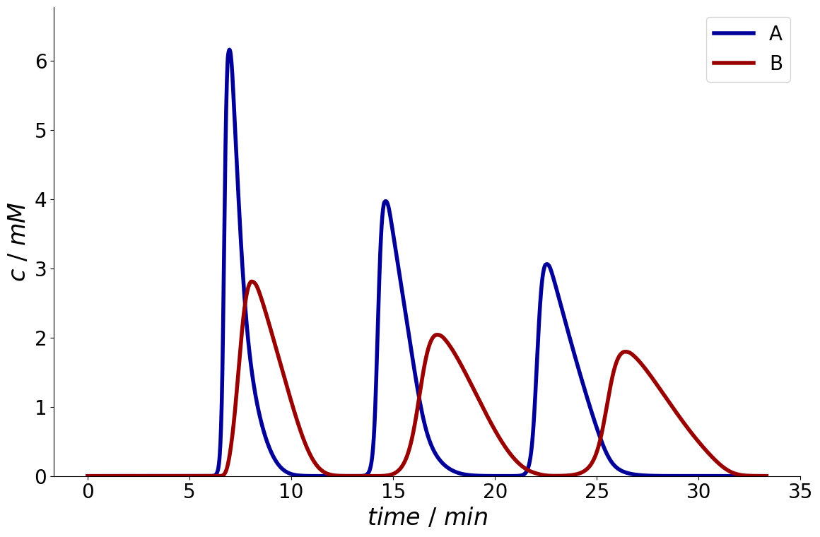
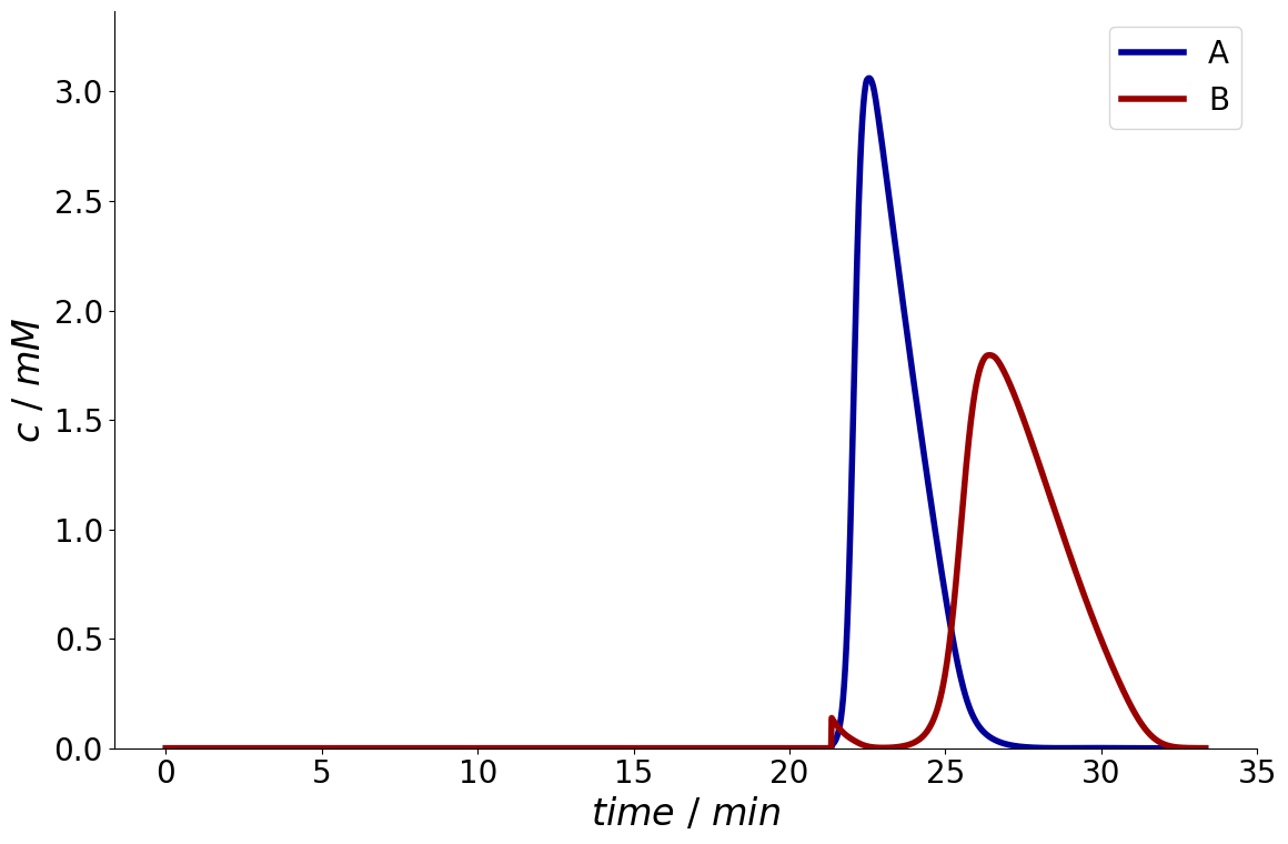
Here, the first plot shows the concentration profile at the column outlet. It is important to note that since part of this profile is recycled, the concentration profile at the system outlet must be considered (second plot) to evaluate the process performance.

if __name__ == '__main__':
    from CADETProcess.simulator import Cadet
    process_simulator = Cadet()

    simulation_results = process_simulator.simulate(process)
    simulation_results.solution.column.outlet.plot()
    simulation_results.solution.outlet.inlet.plot()

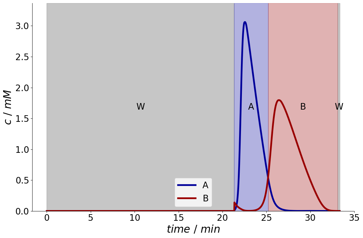
../../_images/c787e7935773a37f21a07f8dbc53247d86a155d886087cd6399fe8b31fa86c01.png

../../_images/7b811cc2b0e84f0670d69233816309a001d448940f0c1ebf43fcb0aa271c46b9.png

Optimize Fractionation Times#

if __name__ == '__main__':
    from CADETProcess.fractionation import FractionationOptimizer
    fractionation_optimizer = FractionationOptimizer()

    fractionator = fractionation_optimizer.optimize_fractionation(
        simulation_results, purity_required=[0.95, 0.95]
    )

    print(fractionator.performance)
    _ = fractionator.plot_fraction_signal()

Performance(mass=array([0.00038081, 0.00038351]), concentration=array([1.8019649 , 0.78253879]), purity=array([0.96352084, 0.95464984]), recovery=array([0.9520315 , 0.95877592]), productivity=array([0.00233828, 0.00235484]), eluent_consumption=array([0.52890639, 0.53265329]) mass_balance_difference=array([-5.53106626e-09, -7.14111788e-08]))

../../_images/6885aa5665455eef685d75bce6a87623fa966ee6f064698a61aecc7334366413.png

Peak Shaving#

The disadvantage of the CLR process is an increased dispersion due to multiple passes through the pump and additional piping.

To improve the overall process performance, the CLR process is often combined with peak shaving. In this process, the initial and final regions of the chromatogram with sufficient purity are “shaved off” during each cycle. Peak shaving can reduce the number of recycling cycles required, since a decreasing amount of components must be pumped across the column.

../../_images/clr_peak_shaving_events.svg — Events for closed-loop recycling process with peak shaving.#

Closed Loop Recycling Process

Contents