Comparing Simulation Results with Reference Data

The CADETProcess.comparison module in CADET-Process offers functionality to quantify the difference between simulations and references, such as other simulations or experiments. The Comparator class allows users to compare the outputs of two simulations or simulations with experimental data. It provides several methods for visualizing and analyzing the differences between the data sets. Users can choose from a range of metrics to quantify the differences between the two data sets, such as sum squared errors or shape comparison.

from CADETProcess.comparison import Comparator
comparator = Comparator()

References

To properly work with CADET-Process, the experimental data needs to be converted to an internal standard. The CADETProcess.reference module provides different classes for different types of experiments. For in- and outgoing streams of unit operations, the ReferenceIO class must be used.

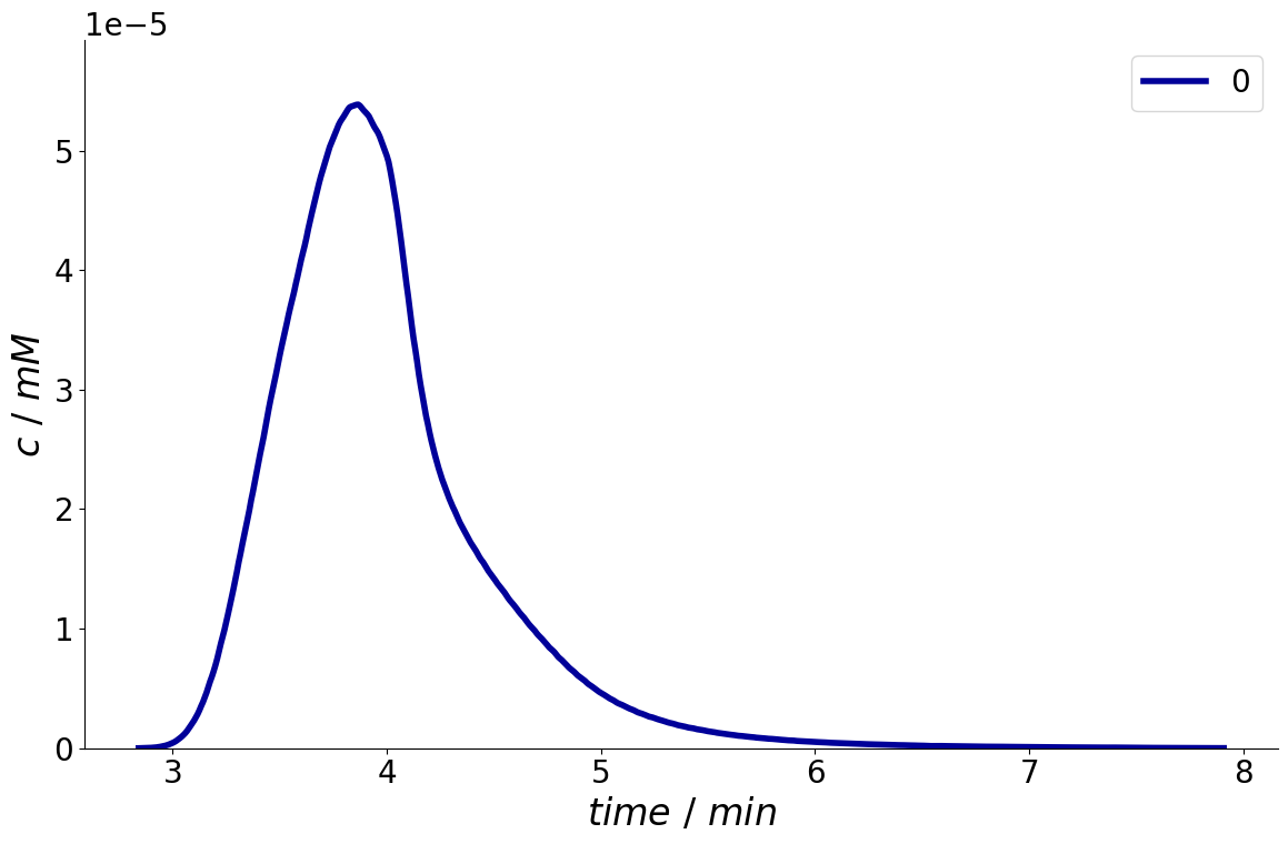
To demonstrate this module, consider a simple tracer pulse injection onto a chromatographic column. The following (experimental) concentration profile is measured at the column outlet. Consider that the time and the data of the experiment are stored in the variables time_experiment, and c_experiment respectively which are simply added to the constructor, together with a name for the reference.

from CADETProcess.reference import ReferenceIO
reference = ReferenceIO('c experiment', time_experiment, c_experiment)

Similarly to the SolutionIO class, the ReferenceIO class also provides a plot method:

_ = reference.plot()

To add the reference to the Comparator, use the add_reference() method.

comparator.add_reference(reference)

Difference Metrics

There are many metrics which can be used to quantify the difference between the simulation and the reference. Most commonly, the sum squared error (SSE) is used. However, SSE is often not an ideal measurement for chromatography. Because of experimental non-idealities like pump delays and fluctuations in flow rate there is a tendency for the peaks to shift in time. This causes the optimizer to favour peak position over peak shape and can lead for example to an overestimation of axial dispersion.

In contrast, the peak shape is dictated by the physics of the physico-chemical interactions while the position can shift slightly due to systematic errors like pump delays. Hence, a metric which prioritizes the shape of the peaks being accurate over the peak eluting exactly at the correct time is preferable. For this purpose, CADET-Process offers a Shape metric [5]. For an overview of all available difference metrics, refer to CADETProcess.comparison.

To add a difference metric, the following arguments need to be passed to the add_difference_metric() method:

• difference_metric: The type of the metric.

• reference: The reference which should be used for the metric.

• solution_path: The path to the corresponding solution in the simulation results.

comparator.add_difference_metric('SSE', reference, 'column.outlet')

Optionally, a start and end time can be specified to only evaluate the difference metric at that slice. This is particularly useful if system noise (e.g. injection peaks) should be ignored or if certain peaks correspond to certain components.

comparator.add_difference_metric(
    'SSE', reference, 'column.outlet', start=3*60, end=6*60
)

<CADETProcess.comparison.difference.SSE at 0x7f1929cbf250>

Reference Model

Next to the experimental data, a reference model needs to be configured. It must include relevant details s.t. it is capable of accurately predicting the experimental system (e.g. tubing, valves etc.). For this example, the full process configuration can be found here.

As an initial guess, the bed porosity is set to \(0.5\), and the axial dispersion to \(1.0 \cdot 10^{-7}\). After process simulation, the evaluate() method is called with the simulation results.

Show code cell content Hide code cell content

from CADETProcess.simulator import Cadet
simulator = Cadet()

from column_transport_parameters import process

process.flow_sheet.column.bed_porosity = 0.5
process.flow_sheet.column.axial_dispersion = 1e-7

simulation_results = simulator.simulate(process)

metrics = comparator.evaluate(simulation_results)
print(metrics)

[2.504752959600517e-06]

The difference can also be visualized:

_ = comparator.plot_comparison(simulation_results)

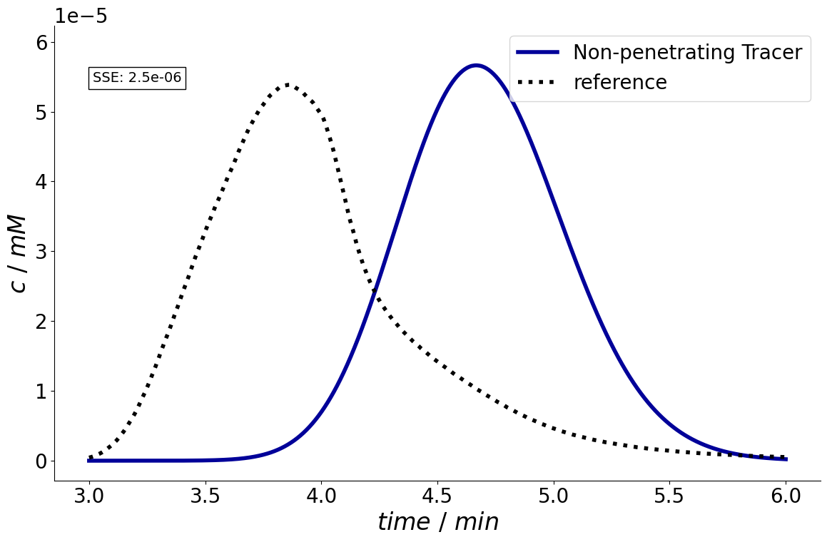
The comparison shows that there is still a large discrepancy between simulation and experiment. Instead of manually adjusting these parameters, an OptimizationProblem can be set up which automatically determines the parameter values. For an example, see Fit Column Transport Parameters.