\[\require{mhchem}\]

Buffer Capacity

For an aqueous solution, the buffer capacity is defined in terms of the change of concentration of acid or base in order to change the pH by one unit. The formal definition of the buffer capacity \(\beta\) is given by the following equation:

\[ \beta = -\frac{dc_a}{d(pH)} \]

The buffer capacity can be resolved into a series of terms, with one term for each active buffer component in the system:

\[ \beta = \beta_{OH^-} + \beta_{H^+} + \sum_{i=1}^{n}\beta_i \]

The terms \(\beta_{OH^-}\) and \(\beta_{H^+}\) account for strong (Arrhenius) acids and bases:

\[\begin{split} \beta_{OH^-} = ln(10) \frac{K_w}{[H^+]} \\ \beta_{H^+} = ln(10) [H^+] \\ \end{split}\]

where \(K_w\) is the autoionization constant of water with a value of \(1.0 \cdot 10^{-14}\). Weak acids and bases are calculated separately. E.g. for monoprotic acids holds:

\[ \beta_i = ln(10) [X_{i, t}] \cdot \frac{K_a [H^+]}{(K_a + [H^+])^2}, \]

where \([X_{i, t}]\) is the total concentration of all species of acid \(i\), and \(K_a\) is the dissociation constant

\[ K_a = 10^{-pKa}. \]

To generalize this for \(n-\text{protic}\) acids, we follow the approach by King and Kester [12],

\[ \beta_i = ln(10) [X_{i, t}] \sum_{j=1}^{n}{\sum_{m=0}^{j-1}{\left(j-m\right)^2 \alpha_j \alpha_m}}, \]

where \(\alpha_j\) is the degree of protolysis for the \(j\text{th}\) dissociation state. For more information, please refer to the original publication.

In CADET-Process, this information can be determined using the equilibria module. Note that these calculations can currently not be performed during simulation. This module rather offers some methods for pre- and post processing.

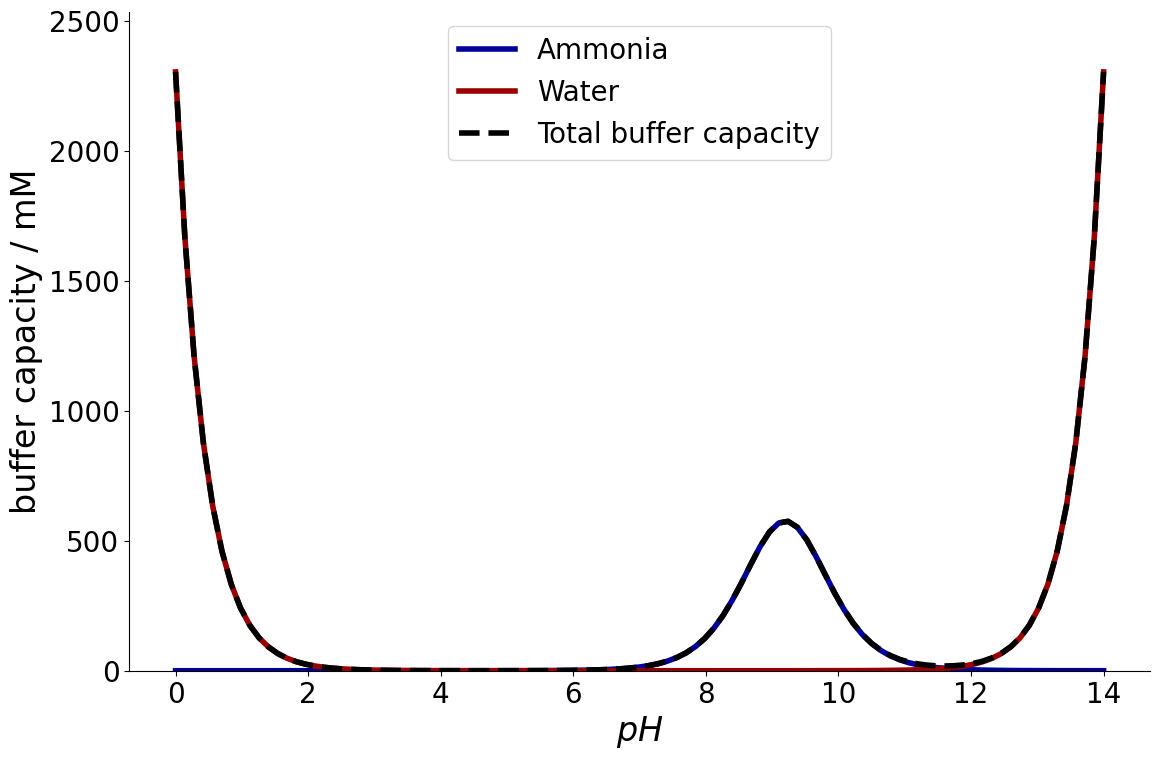
Example Ammonia

To demonstrate this, a \(1~M\) ammonia solution is considered.

First, the ComponentSystem needs to be defined. Please note that for this module to work correctly, H+ needs to be added as an individual component and all deprotonation states need to be added in descending order of their \(pK_a\) value.

from CADETProcess.processModel import ComponentSystem

component_system = ComponentSystem()
component_system.add_component(
    'H+',
    charge=1
)
component_system.add_component(
    'Ammonia',
    species=['NH4+', 'NH3'],
    charge=[1, 0]
)

Then, the MassActionLaw reaction model is defined. The CADETProcess.processModel.MassActionLaw.add_reaction() method expects the following arguments:

• component indices

• stoichiometric coefficients

• forward reaction rate

• backward reaction rate (or, if the reaction is considered quasi-stationary, is_kinetic=False)

If the acid undergoes more than one dissociation reaction, the reactions need to be added with increasing \(pK_a\) values. For more information about configuring reaction models, refer to Chemical Reactions.

from CADETProcess.processModel import MassActionLaw

reaction_system = MassActionLaw(component_system)
reaction_system.add_reaction(
    [0, 1, 2], [-1, 1, 1], 10**(-9.2)*1e3, is_kinetic=False
)

Now, the buffer capacity can be calculated using the CADETProcess.equilibria module. For this purpose, the MassActionLaw model needs to be passed as an argument, as well as a buffer concentration, and the \(pH\) value of interest.

from CADETProcess import equilibria

buffer = [0, 1000, 0]
pH = 7
print(equilibria.buffer_capacity(reaction_system, buffer, pH))

[1.43467153e+01 4.60517019e-04]

The first value is the buffer capacity of the acid, the last value is always the buffer capacity of water. The module provides a function to plot the capacity as a function of pH.

_ = equilibria.plot_buffer_capacity(reaction_system, buffer)

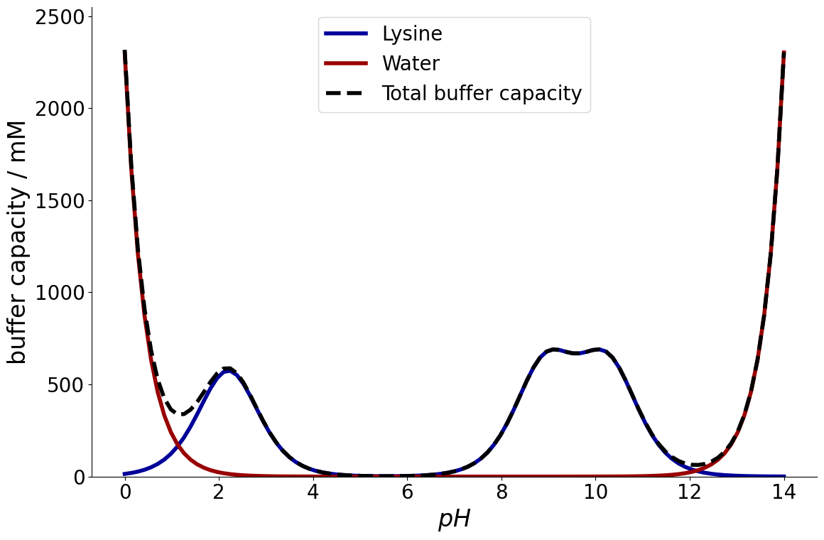
Example Lysine

As in the previous chapter, again as system with lysine is considered:

component_system = ComponentSystem()
component_system.add_component(
    'H+',
)
component_system.add_component(
    'Lysine',
    species=['Lys2+', 'Lys+', 'Lys', 'Lys-'],
)

reaction_system = MassActionLaw(component_system, name='Lysine')
reaction_system.add_reaction(
    [1, 2, 0], [-1, 1, 1], 10**(-2.20)*1e3, is_kinetic=False
)
reaction_system.add_reaction(
    [2, 3, 0], [-1, 1, 1], 10**(-8.90)*1e3, is_kinetic=False
)
reaction_system.add_reaction(
    [3, 4, 0], [-1, 1, 1], 10**(-10.28)*1e3, is_kinetic=False
)

Again, the MassActionLaw model needs to be passed to the CADETProcess.buffer_capacity() function, as well as a buffer concentration, and a corresponding \(pH\):

buffer = [0, 1000, 0, 0, 0]
pH = 7
print(equilibria.buffer_capacity(reaction_system, buffer, pH))
_ = equilibria.plot_buffer_capacity(reaction_system, buffer)

[2.83671767e+01 4.60517019e-04]