Process Simulation

To simulate a Process, a simulator needs to be configured. The simulator translates the Process configuration into the API of the corresponding external simulator. As of now, only CADET has been adapted but in principle, other simulators can be also implemented. CADET needs to be installed separately for example using mamba.

mamba install -c conda-forge cadet

For more information on CADET, refer to the CADET Documentation

Instantiate Simulator

First, Cadet needs to be imported. If no path is specified in the constructor, CADET-Process will try to autodetect the CADET installation.

from CADETProcess.simulator import Cadet
process_simulator = Cadet()

If a specific version of CADET is to be used, add the install path to the constructor:

process_simulator = Cadet(install_path='/path/to/cadet/executable')

To verify that the installation has been found correctly, call the check_cadet() method:

process_simulator.check_cadet()

Test simulation completed successfully

True

Simulator Parameters

For all simulator parameters, reasonable default values are provided but there might be cases where those might need to be changed.

Time Stepping

CADET uses adaptive time stepping. That is, the time step size is dynamically adjusted based on the rate of change of the variables being simulated. This balances the tradoff between simulation accuracy and computational efficiency by reducing the time step size when the error estimate is larger than a specified tolerance and increasing it when the error estimate is smaller.

After simulation, the solution is interpolated and stored in an array. To change the resolution of that solution, set the time_resolution attribute.

print(process_simulator.time_resolution)

1.0

Note that changing this value does not have an effect on the accuracy of the solution. To change error tolerances, modify the attributes of the SolverTimeIntegratorParameters

print(process_simulator.time_integrator_parameters)

<CADETProcess.simulator.cadetAdapter.SolverTimeIntegratorParameters object at 0x7f1a80ed9550>

Most notably, abstol and abstol might need to be adapted in cases where high accuracy is required. For more information, see SolverTimeIntegratorParameters and refer to the CADET Documentation.

Solver Parameters

The SolverParameters stores general parameters of the solver.

print(process_simulator.solver_parameters)

<CADETProcess.simulator.cadetAdapter.SolverParameters object at 0x7f1a81337550>

Most notably, nthreads defines the number of threads with which the simulation is parallelized. For more information, see also CADET Documentation.

Model Solver Parameters

The ModelSolverParameters stores general parameters of the model solver.

print(process_simulator.solver_parameters)

<CADETProcess.simulator.cadetAdapter.SolverParameters object at 0x7f1a81337550>

For more information, see also CADET Documentation.

Simulate Processes

To run the simulation, pass the Process as an argument to the simulate() method. For this example, consider a simple batch-elution example.

simulation_results = process_simulator.simulate(process)

Sometimes simulations can take a long time to finish. To limit their runtime, add a timeout argument with the maximum simulation time in seconds.

simulation_results = process_simulator.simulate(process, timeout=300)

Simulation Results

The SimulationResults object contains the results of the simulation. This includes:

• exit_code: Information about the solver termination.

• exit_message: Additional information about the solver status.

• time_elapsed: Execution time of simulation.

• n_cycles: Number of cycles that were simulated.

• solution: Complete solution of all cyles.

• solution_cycles: Solution of individual cycles.

In the solution attribute, SolutionBase objects for each unit operation are stored. By default, the inlet and outlet of each unit are stored. To also include other solution types such as bulk or solid phase, this needs to be configured before simulation in the corresponding solutionRecorder. For more information refer to Unit Operation Models.

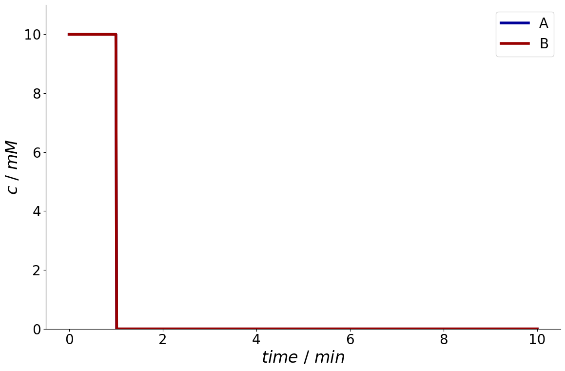
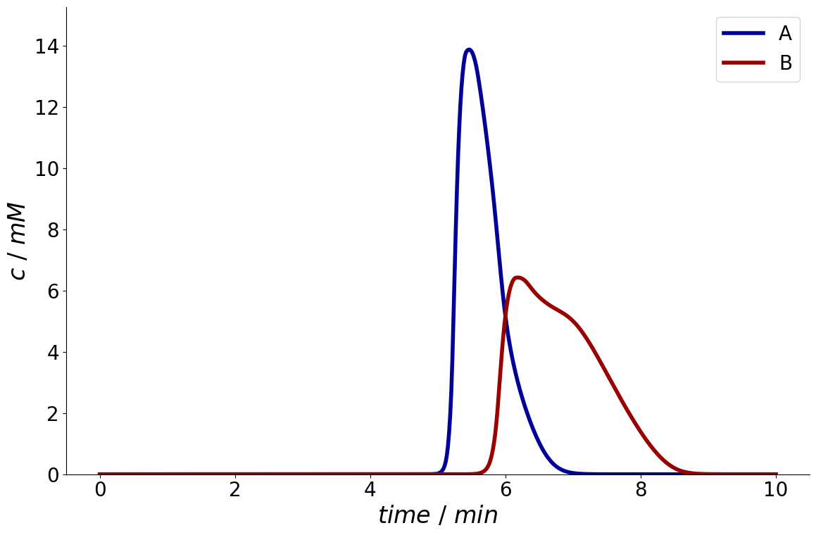
All solution objects provide plot methods. For example, the plot() method of the SolutionIO class which is used to store the inlets and outlets of unit operations plots the concentration profile over time.

_ = simulation_results.solution.column.inlet.plot()
_ = simulation_results.solution.column.outlet.plot()

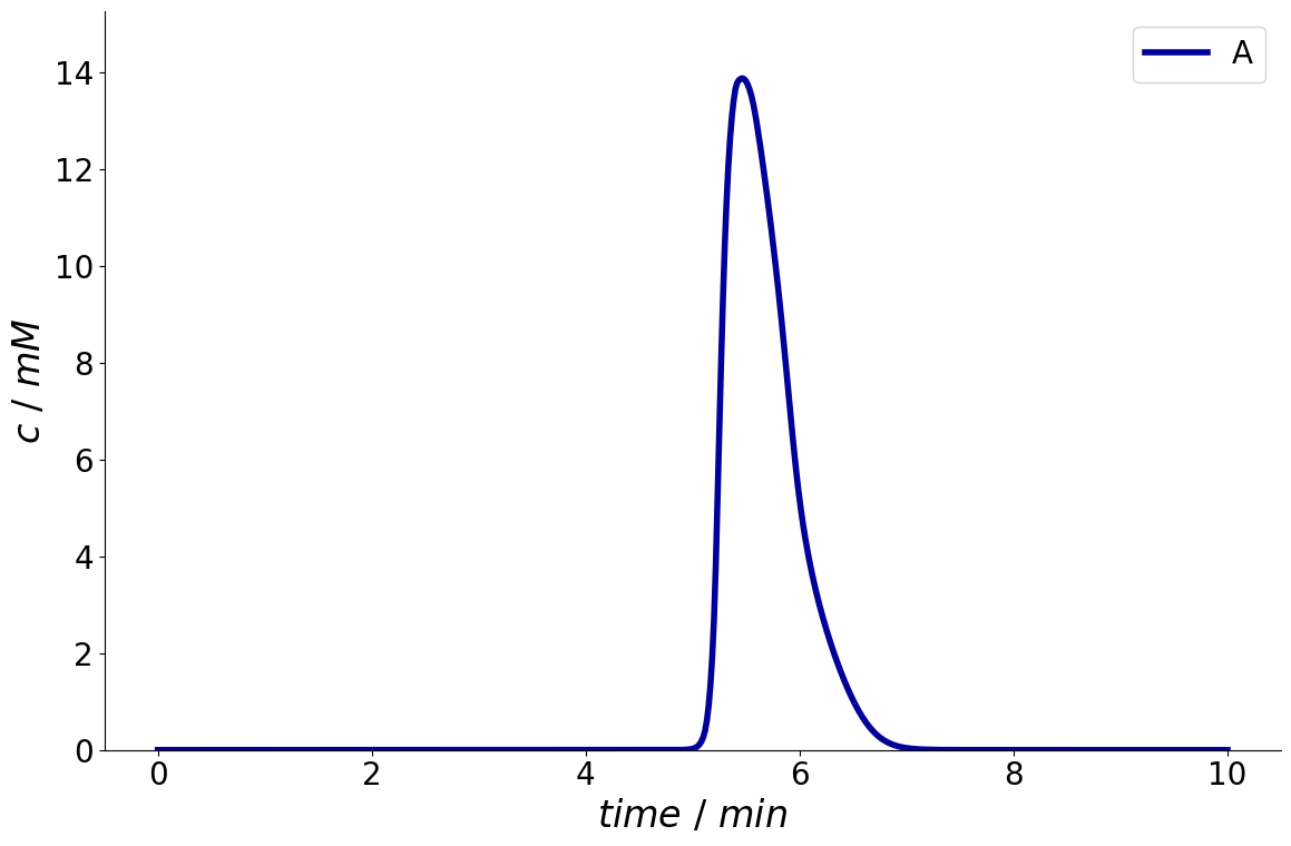
It is also possible to only plot specific components by specifying a list of component names.

_ = simulation_results.solution.column.outlet.plot(components=['A'])

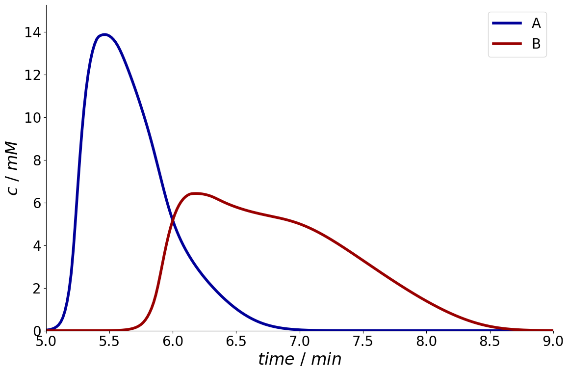
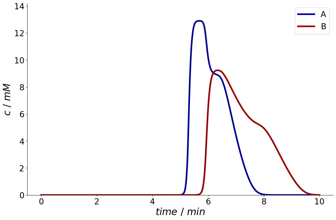
Moreover, a time interval can be specified with arguments start and end.

_ = simulation_results.solution.column.outlet.plot(start=5*60, end=9*60)

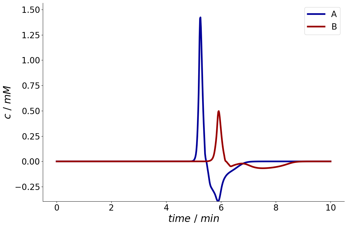
The SolutionIO also provides access to the derivative and antiderivative of the solution which in turn are also SolutionIO objects.

derivative = simulation_results.solution.column.outlet.derivative
_ = derivative.plot()

If parameter sensitivities have been specified (see Parameter Sensitivities), the resulting sensitivities are also stored in sensitivity attribute. This dict contains an entry for every sensitivity. For each of those entries, the sensitivity is stored for each of the unit operations as defined in the corresponding CADETProcess.processModel.solutionRecorder (see Solution Recorder). For example, if column.total_porosity has been defined, the structure would look like the following:

print(simulation_results.sensitivity.keys())
print(simulation_results.sensitivity['column.total_porosity'].keys())
print(simulation_results.sensitivity['column.total_porosity'].column.keys())

dict_keys(['column.total_porosity'])
dict_keys(['feed', 'eluent', 'column', 'outlet'])
dict_keys(['inlet', 'outlet'])

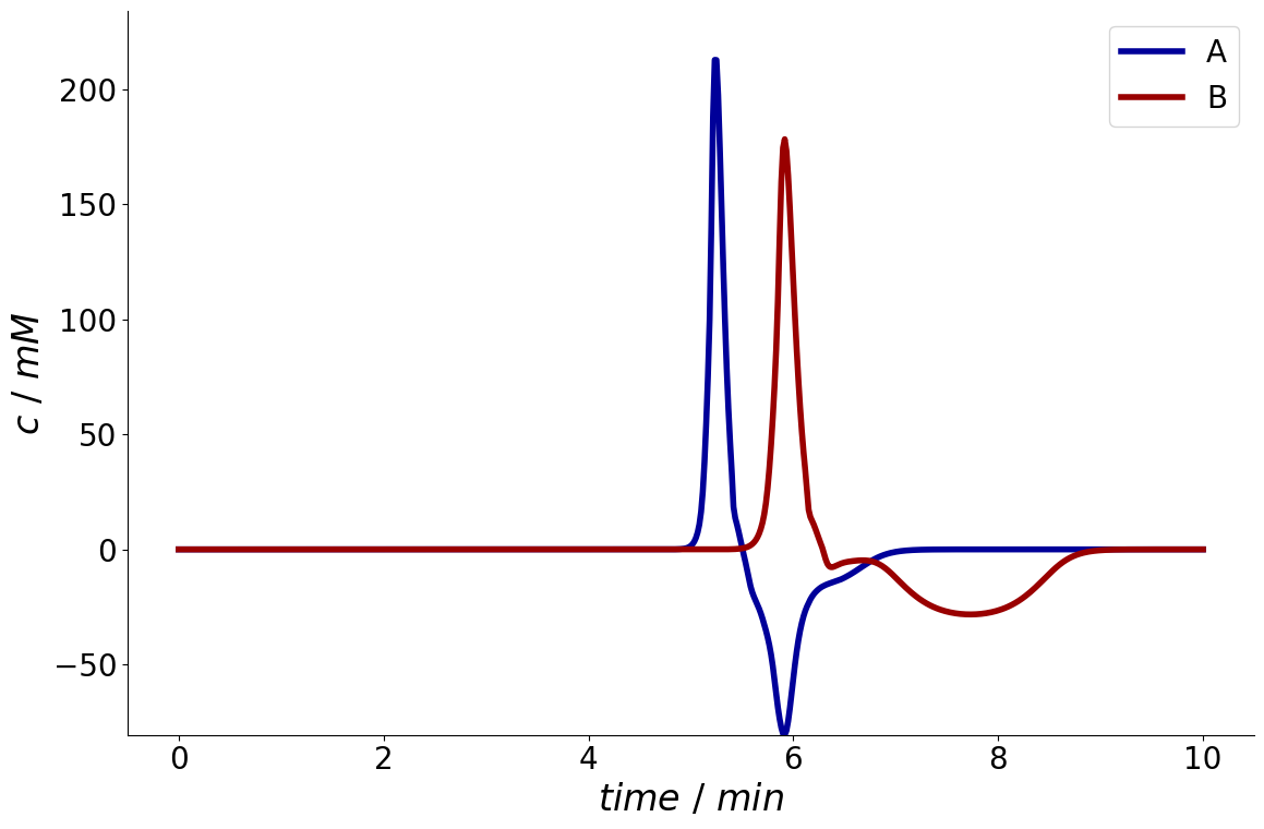
Here, the outlet entry again is a SolutionIO which can be plotted.

_ = simulation_results.sensitivity['column.total_porosity'].column.outlet.plot()

Cyclic Stationarity

Preparative chromatographic separations are operated in a repetitive fashion. In particular processes that incorporate the recycling of streams, like steady-state-recycling (SSR) or simulated moving bed (SMB), have a distinct startup behavior that takes multiple cycles until a periodic steady state is reached. But also in conventional batch chromatography several cycles are needed to attain stationarity in optimized situations where there is a cycle-to-cycle overlap of the elution profiles of consecutive injections. However, it is not known beforehand how many cycles are required until cyclic stationarity is established.

For this reason, the simulator can simulate a Process for a fixed number of cycles, or continue simulating until the StationarityEvaluator (see Figure: Framework Overview) confirms that cyclic stationarity is reached. Different criteria can be specified such as the maximum deviation of the concentration profiles or the peak areas of consecutive cycles [1]. The simulation terminates if the corresponding difference is smaller than a specified value. For the evaluation of the process (see Product Fractionation), only the last cycle is examined, as it yields a representative Performance of the process in all later cycles.

To demonstrate this concept, consider a SSR process (see here for the full process configuration).

A first strategy is to simulate multiple cycles at once. For this purpose, we can specify n_cycles for the simulator.

process_simulator.n_cycles = 10
simulation_results = process_simulator.simulate(process)
_ = simulation_results.solution.column.outlet.plot()

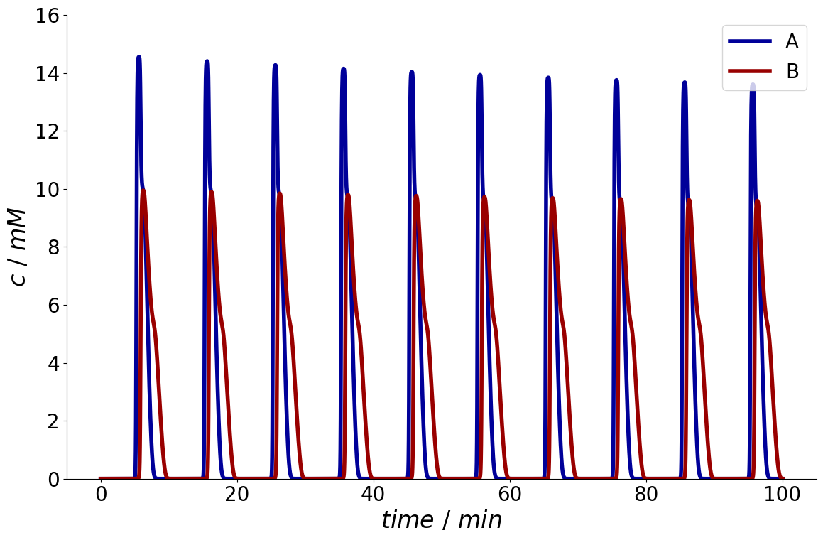
However, it is hard to anticipate, when steady state is reached. To automatically simulate until stationarity is reached, a StationarityEvaluator needs to be configured.

from CADETProcess.stationarity import StationarityEvaluator

evaluator = StationarityEvaluator()

In this example, the relative change in the area of the solution (i.e. the integral of the chromatogram) of succeeding cycles should be compared. For this purpose, a RelativeArea criterion is configured and added to the Evaluator. The threshold is set to 1e-3 indicating that the change in area must be smaller than \(0.1~\%\).

from CADETProcess.stationarity import RelativeArea

criterion = RelativeArea()
criterion.threshold = 1e-3

evaluator.add_criterion(criterion)

Then, the evaluator is added to the simulator and the evaluate_stationarity flag in the simulator is set to True.

process_simulator.stationarity_evaluator = evaluator
process_simulator.evaluate_stationarity = True

To prevent running too many simulations (e.g. when stationarity is never reached), it is possible to limit the maximum number of cycles that are evaluated:

process_simulator.n_cycles_max = 100

In addition, because stopping the simulation, evaluating the stationarity, and then restarting the simulation comes with some overhead, it is also possible to set a minimum number of cycles that are simulated between evaluations:

process_simulator.n_cycles_min = 10

Now the simulator runs until stationarity is reached.

simulation_results = process_simulator.simulate(process)
_ = simulation_results.solution.column.outlet.plot()

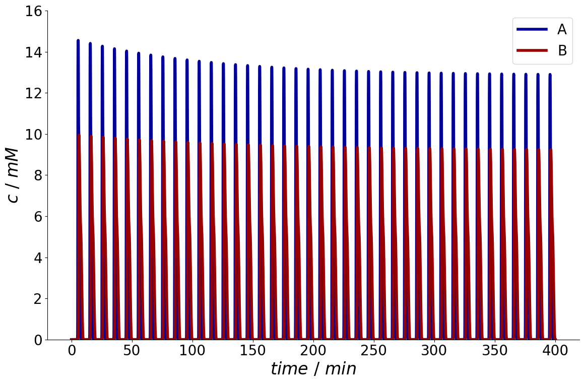
The number of cycles is stored in the simulation results.

print(simulation_results.n_cycles)

40

It is possible to access the solution of any of the cycles. For the last cycle, use the index -1.

_ = simulation_results.solution_cycles.column.outlet[-1].plot()

Note that the simulator by default already contains a preconfigured StationarityEvaluator. Usually, it is sufficient to only set the evaluate_stationarity flag.