
Parameter Spaces and Sampling#
The ParameterSpace defines a feasible domain and writes parameter values into model objects.
It is the foundation that OptimizationProblem builds on, but it is also useful on its own: design-of-experiments studies, surrogate training data, and sensitivity screenings all need feasible parameter samples without any optimizer involved.
This guide shows how to build a space, assign values, and draw samples with different strategies.
Defining a Parameter Space#
A parameter space connects parameter declarations to attributes of one or more evaluation objects.
Any Python object with writable attributes works; in practice this is usually a Process.
from dataclasses import dataclass

from CADETProcess.parameter_space import ParameterSpace, RangedParameter


@dataclass
class Column:
    length: float = 0.5
    diameter: float = 0.05


column = Column()

space = ParameterSpace()
space.add_evaluation_object(column)
space.add_parameter(
    RangedParameter("length", float, lb=0.1, ub=1.0), path="length"
)
space.add_parameter(
    RangedParameter("diameter", float, lb=0.01, ub=0.2), path="diameter"
)
space
ParameterSpace(n_variables=2, n_parameters=2, evaluation_objects=1)
Each RangedParameter declares a name, a type, and bounds; the path tells the space where the value lives on the evaluation object.
Named Assignments#
Values are written as named assignments, plain dictionaries mapping parameter names to physical values.
space.set_values({"length": 0.75, "diameter": 0.04})
column
Column(length=0.75, diameter=0.04)
Reading goes through get_value().
space.get_value("length")
0.75
Dependencies#
A dependent parameter is computed from other parameters via a transform. The assignment then only contains the independent parameters; the space resolves the rest.
length, diameter = space.independent_parameters
space.add_dependency(diameter, [length], transform=lambda le: le / 10)

space.set_values({"length": 0.6})
column
Column(length=0.6, diameter=0.06)
resolve() returns the full assignment without writing anything.
space.resolve({"length": 0.6})
{'length': 0.6, 'diameter': 0.06}
Linear Constraints#
Linear inequality constraints of the form \(A x \le b\) restrict the feasible domain beyond the box bounds.
from CADETProcess.parameter_space import LinearConstraint

flow = ParameterSpace()
flow.add_evaluation_object(Column())
q_load = RangedParameter("q_load", float, lb=0.0, ub=10.0)
q_elute = RangedParameter("q_elute", float, lb=0.0, ub=10.0)
flow.add_parameter(q_load, path="length")
flow.add_parameter(q_elute, path="diameter")

# q_load must not exceed q_elute
flow.add_linear_constraint(LinearConstraint([q_load, q_elute], lhs=[1, -1], b=0))
Sampling#
sample() draws feasible points as named assignments.
All samples respect bounds, linear constraints, and dependencies; constraints referencing dependent parameters are enforced by rejection.
flow.sample(3, seed=42)
[{'q_load': 3.8831707228758643, 'q_elute': 7.82768309118836},
 {'q_load': 2.3658788906415475, 'q_elute': 3.086857406426368},
 {'q_load': 1.4453330847790702, 'q_elute': 9.748866762397633}]
Passing a seed makes the draw reproducible; unseeded calls use a fresh random seed.
Sampling Strategies#
Three sampler backends are available, all sharing the same interface.
HopsySampler draws uniformly from the constrained polytope via Markov chain Monte Carlo (hopsy).
It is the default used by space.sample() and the only correct choice when linear constraints are present.
LatinHypercubeSampler and SobolSampler produce space-filling designs for box-bounded spaces, the right tool for surrogate training data and design-of-experiments.
Both raise when linear constraints are present, because filtering a quasi-Monte-Carlo design destroys its uniformity guarantees.
from CADETProcess.parameter_space import HopsySampler, LatinHypercubeSampler

box = ParameterSpace()
box.add_evaluation_object(Column())
box.add_parameter(RangedParameter("x_0", float, lb=0.0, ub=1.0), path="length")
box.add_parameter(RangedParameter("x_1", float, lb=0.0, ub=1.0), path="diameter")

uniform = HopsySampler(pool_size=2000).sample(box, 64, seed=0)
lhs = LatinHypercubeSampler().sample(box, 64, seed=0)
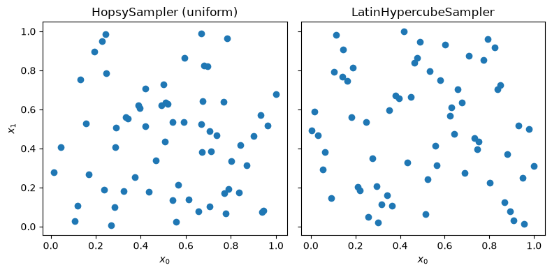
The difference is visible directly: uniform draws cluster and leave gaps, the Latin Hypercube covers every stratum exactly once per dimension.
import matplotlib.pyplot as plt

fig, axes = plt.subplots(1, 2, figsize=(8, 4), sharey=True)
for ax, samples, title in [
    (axes[0], uniform, "HopsySampler (uniform)"),
    (axes[1], lhs, "LatinHypercubeSampler"),
]:
    ax.scatter([s["x_0"] for s in samples], [s["x_1"] for s in samples])
    ax.set_title(title)
    ax.set_xlabel(r"$x_0$")
axes[0].set_ylabel(r"$x_1$")
fig.tight_layout()
Integer and Categorical Parameters#
Integer parameters are declared with int as the parameter type; sampled assignments carry proper int values.
Categorical parameters are declared as ChoiceParameter and have no numeric position; samplers draw them alongside the numeric dimensions.
The quasi-Monte-Carlo samplers treat each categorical parameter as an extra design dimension, so category counts come out balanced.
from CADETProcess.parameter_space import ChoiceParameter

mixed = ParameterSpace()
mixed.add_evaluation_object(Column())
mixed.add_parameter(RangedParameter("n_plates", int, lb=10, ub=100), path="length")
mixed.add_parameter(ChoiceParameter("resin", ["A", "B"]))

samples = LatinHypercubeSampler().sample(mixed, 10, seed=0)
samples[:3]
[{'n_plates': 49, 'resin': 'A'},
 {'n_plates': 64, 'resin': 'A'},
 {'n_plates': 75, 'resin': 'B'}]
[s["resin"] for s in samples].count("A")
5
Chebyshev Center#
The Chebyshev center is the center of the largest ball inscribed in the constrained polytope, a robust interior starting point.
from CADETProcess.parameter_space import chebyshev_center

chebyshev_center(flow)
{'q_load': 2.928932188134525, 'q_elute': 7.0710678118654755}
Note
The center is undefined for spaces with categorical parameters and raises in that case.
Linear constraints referencing dependent parameters cannot enter the polytope; they are dropped with a warning and the returned point is verified against them, so the result is either feasible or a ValueError.
Note
The center is the center of the largest inscribed ball, not the midpoint of the box bounds.
In an anisotropic space (e.g. one parameter spanning 1 to 600, another spanning 1e-8 to 1e-4), the ball’s radius is capped by the narrowest dimension, leaving it free to slide along the wider ones: the center can land close to a bound on the wide dimension rather than near its middle.
Use with OptimizationProblem#
create_initial_values() accepts any sampler via the sampler argument, which is useful when the initial population doubles as a space-filling design.
from CADETProcess.optimization import OptimizationProblem

problem = OptimizationProblem("sampling_demo", use_diskcache=False)
problem.add_variable("x_0", lb=0, ub=8)
problem.add_variable("x_1", lb=0, ub=1)

problem.create_initial_values(8, seed=1, sampler=LatinHypercubeSampler())
array([[7.48817838, 0.88119204],
       [6.85584039, 0.38141882],
       [2.68816855, 0.32208419],
       [0.17229741, 0.57385011],
       [4.45040631, 0.12155511],
       [5.24648689, 0.80773209],
       [1.67026828, 0.65144641],
       [3.69680517, 0.19331276]])