Instruments

The instruments module provides ready-made LC system flow sheet templates and experiment process classes. Rather than manually assembling a FlowSheet and adding events by hand, you pick a pre-built template or compose phases declaratively.

The design follows the same two-step pattern as plain CADET-Process objects: construct the flow sheet first, then pass it to the process. This chapter builds up in that order: the flow sheet topology, then the valve positions and phase primitives, then PhasedProcess, which composes them, and finally the protocol templates that specialize it. To run a standard protocol without the underlying details, skip ahead to Process templates.

LC system topology

All templates share the same physical topology, modelled by LCFlowSheet. The topology and valve nomenclature follow typical preparative LC instruments such as the Äkta (Cytiva) and Knauer Azura series.

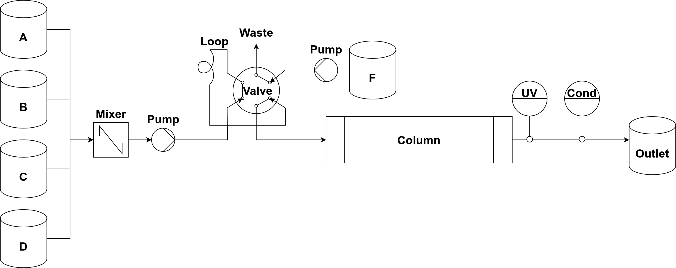
Physical topology of the modeled LC system. Internally, each tubing segment, the mixer, and the sample loop are represented as explicit unit operations with configurable dimensions; see the units table below. Pumps and inline detectors are not modeled as separate units: flow rates are set directly on the inlet units.

Inlets

Name	Purpose
buffer_a to buffer_d	Eluent reservoirs; flow through the mixer for gradient formation
feed_inlet	Feed inlet; connects directly to the sample loop

Internal units

Name	Model	Purpose
mixer	Cstr	Mixes buffers A to D
tubing_pre_injection	TubularReactor	Dead volume between mixer and injection point
sample_loop	TubularReactor	Injection loop; content set as initial condition
tubing_pre_column	TubularReactor	Pre-column dead volume
column	configurable	Chromatographic column
tubing_post_column	TubularReactor	Post-column dead volume
tubing_detectors	TubularReactor	Detector cell dead volume

Outlets: outlet (product) and waste (for loop loading and pump waste routing).

from CADETProcess.processModel import ComponentSystem, LumpedRateModelWithPores, Linear
from CADETProcess.instruments import LCFlowSheet

cs = ComponentSystem(["Salt", "Protein"])
Q = 1.0e-8  # m³/s

fs = LCFlowSheet(
    cs,
    sample_loop_volume=50e-9,
    sample_loop_diameter=0.75e-3,
    ColumnModel=LumpedRateModelWithPores,
    BindingModel=Linear,
)
print("units:", [u.name for u in fs.units])

units: ['buffer_a', 'buffer_b', 'buffer_c', 'buffer_d', 'feed_inlet', 'mixer', 'tubing_pre_injection', 'sample_loop', 'tubing_pre_column', 'column', 'tubing_post_column', 'tubing_detectors', 'outlet', 'waste']

Units can be excluded from the flow path to characterize the system sequentially, starting from the simplest configuration and adding components one at a time. The bypass flow sheet below keeps the sample loop but removes the column and surrounding tubing; it is reused throughout the rest of this chapter.

fs_no_col = LCFlowSheet(
    cs,
    sample_loop_volume=50e-9,
    sample_loop_diameter=0.75e-3,
    bypass_units=["tubing_pre_column", "column", "tubing_post_column", "tubing_detectors"],
)
print("units:", [u.name for u in fs_no_col.units])

units: ['buffer_a', 'buffer_b', 'buffer_c', 'buffer_d', 'feed_inlet', 'mixer', 'tubing_pre_injection', 'sample_loop', 'outlet', 'waste']

Valve positions

Two pumps feed the system. SyP (system pump) is the buffer line: buffers A to D flow through the mixer into tubing_pre_injection. SaP (sample pump) is the feed line: feed_inlet connects directly to the sample loop (or first_unit when no loop is present).

A valve position sets where each pump’s output goes and whether the sample loop sits in the active flow path. Four named positions are available, with two aliases:

Position	Alias	SyP (tubing_pre_injection)	SaP / loop	Requires loop
"run"		→ first_unit	→ waste	no
"load"		→ first_unit	→ loop → waste	yes (degrades to "run")
"inject"	"sample_pump_waste"	→ loop → first_unit	→ waste	yes (degrades to "run")
"direct_inject"	"system_pump_waste"	→ waste	→ first_unit	no

The default position before the first event is "run". Positions that require a loop degrade to "run" when the flow sheet has none, so a protocol written for a full system still runs on a bypass configuration.

Phases and valve events

A process is built from two primitives: phases, which set the flow over an interval, and valve events, which switch the flow path at an instant.

Phases

A Phase specifies a duration, a flow rate, and the buffer composition over that interval. Passing only a start composition gives a step (constant composition); passing a different end composition gives a linear gradient. The feed inlet appears as key "F" and cannot be mixed with buffers A to D in the same phase.

from CADETProcess.instruments import Phase

gradient = Phase(400.0, Q, {"A": 1.0}, {"B": 1.0})  # A → 0, B → 1 over 400 s
wash     = Phase(200.0, Q, {"A": 1.0})              # step: constant 100 % A
feed     = Phase(60.0,  Q, {"F": 1.0})              # sample via feed inlet
print("gradient end:", gradient.composition_end, "| wash end:", wash.composition_end)

gradient end: {'B': 1.0} | wash end: {'A': 1.0}

Valve events

A ValveEvent is an instantaneous change to one of the positions above. A single position change affects several units at once (the loop and the pre-injection tubing switch together); the coupled events stay linked, so moving the primary event, e.g. during optimization, propagates to the rest.

There are two ways to schedule valve events. The declarative form places a ValveEvent in a PhasedProcess step sequence, where its time follows from the cumulative phase durations (shown in the next section). The imperative form calls add_valve_event() on any LCProcess at an explicit time.

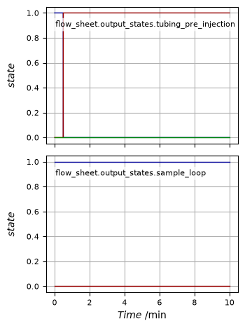
A single injection: push the loop contents onto the flow path at t=0, then return to run once the loop is cleared.

from CADETProcess.instruments import LCProcess

single = LCProcess("single_inj", fs_no_col)
single.cycle_time = 600.0
single.add_valve_event("inject", t=0.0)
single.add_valve_event("run",    t=30.0)
single.plot_events();

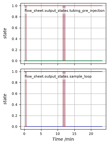
Successive injections reload the loop during the run, something the fixed-protocol templates cannot express.

multi = LCProcess("multi_inj", fs_no_col)
multi.cycle_time = 1400.0
multi.add_valve_event("inject", t=0.0)    # first injection: loop → flow path
multi.add_valve_event("load",   t=30.0)   # feed_inlet refills the loop during the run
multi.add_valve_event("inject", t=700.0)  # second injection
multi.add_valve_event("load",   t=730.0)  # reload again
multi.plot_events();

For system equilibration before the column, system_pump_waste (alias of direct_inject) routes the system pump to waste while the path settles, then a run event switches back.

Composing a process with PhasedProcess

PhasedProcess composes a steps list of Phase and ValveEvent objects into a complete process; the cycle time is the sum of the phase durations. It is the base class for all the protocol templates in the next section.

from CADETProcess.instruments import PhasedProcess

steps = [
    Phase(200.0, Q, {"A": 1.0}),                 # wash: 100 % A
    Phase(400.0, Q, {"A": 1.0}, {"B": 1.0}),     # gradient: A → 0, B → 1
    Phase(100.0, Q, {"A": 1.0}),                 # final wash
]
custom = PhasedProcess("custom", fs_no_col, steps)
print("cycle_time:", custom.cycle_time, "s")
print("events:", [e.name for e in custom.events])
custom.plot_events();

cycle_time: 700.0 s
events: ['phase_0_A', 'phase_0_B', 'phase_1_A', 'phase_1_B', 'phase_2_A', 'phase_2_B']

Interleaving valve events reproduces the single injection from above, now declaratively:

from CADETProcess.instruments import ValveEvent

pulse_steps = [
    ValveEvent("inject"),
    Phase(30.0,  Q, {"A": 1.0}),
    ValveEvent("run"),
    Phase(570.0, Q, {"A": 1.0}),
]
pulse_proc = PhasedProcess("pulse", fs_no_col, pulse_steps)
pulse_proc.plot_events();

The declarative form derives each valve event’s time from the phase durations that precede it, so resizing or reordering phases shifts the events automatically. The imperative add_valve_event form is the escape hatch when events must sit at explicit, protocol-independent times.

Process templates

The templates below are PhasedProcess subclasses that fill in the step sequence for a standard protocol. Each takes a pre-constructed LCFlowSheet as its second argument.

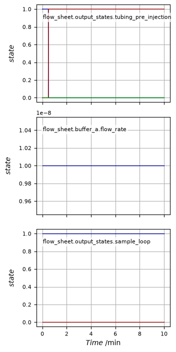
PulseInjection

The system is pre-equilibrated with buffer A. The sample loop content is injected at t=0 and washed through with buffer A.

from CADETProcess.instruments import PulseInjection

pulse = PulseInjection(
    "pulse", fs_no_col,
    c_buffer_a=[0.0, 0.0],
    c_sample=[0.0, 1.0],
    cycle_time=600.0,
    flow_rate=Q,
)
print("cycle_time:", pulse.cycle_time, "s")
print("buffer_a flow rate:", pulse.flow_sheet.buffer_a.flow_rate[0], "m³/s")
pulse.plot_events();

cycle_time: 600.0 s
buffer_a flow rate: 1e-08 m³/s

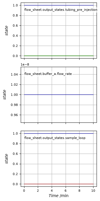
Step

A single-phase switch of the running buffer from A to B at t=0, with no sample injected. The buffer B front passes through the system unretained, so its response measures dead volumes and mixing dynamics. For injecting and eluting a sample with a step gradient, use StepElution instead.

from CADETProcess.instruments import Step

step = Step(
    "step", fs_no_col,
    c_buffer_a=[0.0, 0.0],
    c_buffer_b=[1000.0, 0.0],
    cycle_time=800.0,
    flow_rate=Q,
)
step.plot_events();

LWE

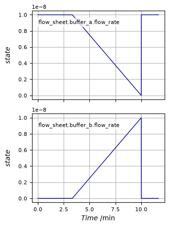
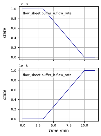
Load-wash-elute with a linear salt gradient. After the wash phase, buffer B ramps up linearly while buffer A ramps down.

from CADETProcess.instruments import LWE

lwe = LWE(
    "lwe", fs,
    c_buffer_a=[20.0, 0.0],
    c_buffer_b=[1000.0, 0.0],
    c_sample=[20.0, 1.0],
    delta_t_wash=200.0,
    delta_t_elute=400.0,
    delta_t_final_wash=100.0,
    flow_rate_wash=Q,
)
print("cycle_time:", lwe.cycle_time, "s")
lwe.plot_events();

cycle_time: 700.0 s

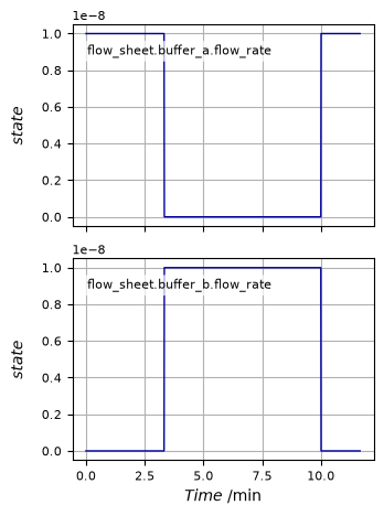
StepElution

A full load-wash-elute protocol like LWE, but the elution uses an instantaneous step to buffer B instead of a linear gradient. Unlike Step, it injects the sample loop contents and runs wash and final-wash phases around the elution step.

from CADETProcess.instruments import StepElution

se = StepElution(
    "se", fs,
    c_buffer_a=[20.0, 0.0],
    c_buffer_b=[1000.0, 0.0],
    c_sample=[20.0, 1.0],
    delta_t_wash=200.0,
    delta_t_elute=400.0,
    delta_t_final_wash=100.0,
    flow_rate_wash=Q,
)
print("cycle_time:", se.cycle_time, "s")
se.plot_events();

cycle_time: 700.0 s

Breakthrough

Sample is loaded continuously from t=0 until the column saturates and breaks through at the outlet, which measures the dynamic binding capacity. Unlike Step, the sample is delivered through the feed inlet (feed_inlet) by default rather than as a change of running buffer, and there is no elution phase. Pass sample_buffer="B" (or any key A to D) to deliver the sample through a main buffer line instead.

from CADETProcess.instruments import Breakthrough

bt = Breakthrough(
    "bt", fs,
    c_sample=[20.0, 1.0],
    flow_rate=Q,
    cycle_time=600.0,
)
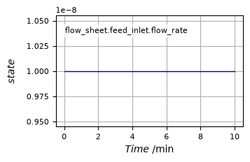
print("feed flow rate:", bt.flow_sheet.feed_inlet.flow_rate[0], "m³/s")
bt.plot_events();

feed flow rate: 1e-08 m³/s