Signal Calibration

The calibration module converts raw detector signals carried by ReferenceIO objects into physical concentration units. All functions return a new ReferenceIO and leave the input unchanged. A typical workflow applies two steps in sequence: baseline correction to remove drift, followed by a calibration step to convert signal units to concentration.

Choosing a calibration method:

• Known injected amount (mol or mass): normalize_area()

• Known molar extinction coefficient: apply_beer_lambert()

• Multiple absorbing species at multiple wavelengths: deconvolve_extinction()

• Empirical detector response or non-UV detectors: fit_polynomial() + apply_polynomial_calibration()

import numpy as np
import matplotlib.pyplot as plt
from CADETProcess.reference import ReferenceIO
from CADETProcess.calibration import (
    crop,
    correct_baseline,
    normalize_area,
    correct_baseline_and_normalize,
    fit_polynomial,
    apply_polynomial_calibration,
    apply_beer_lambert,
    deconvolve_extinction,
)

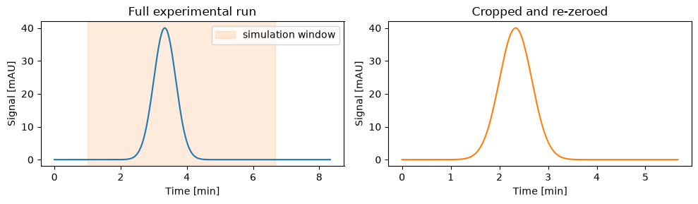
Cropping to the simulation window

An experimental run typically extends beyond the simulated process: the pump may need time to stabilize before injection starts, and a wash step at the end is not part of the simulation. crop() extracts the relevant portion and re-zeros the time axis so it aligns with simulation time starting at \(t = 0\).

time_full = np.linspace(0, 500, 5001)
signal_full = (40 * np.exp(-0.5 * ((time_full - 200) / 20) ** 2)).reshape(-1, 1)
raw_full = ReferenceIO("UV 280 nm (full run)", time_full, signal_full, flow_rate=1e-6)

# Injection started at t = 60 s; wash step ended at t = 400 s
cropped = crop(raw_full, start=60, end=400)

Baseline correction

Detector signals often carry a slow linear drift caused by temperature changes, gradient-induced refractive index shifts, or lamp instability. correct_baseline() estimates a linear baseline from the lowest-intensity points in the signal and subtracts it pointwise.

time = np.linspace(0, 900, 9001)  # seconds (15 min run)

drift = 5.0 + 0.02 * time  # mAU
ghost = 15 * np.exp(-0.5 * ((time - 120) / 15) ** 2)  # ghost peak at ~2 min
peak  = 80 * np.exp(-0.5 * ((time - 600) / 30) ** 2)  # main peak at ~10 min
signal = (drift + ghost + peak).reshape(-1, 1)

raw = ReferenceIO("UV 280 nm", time, signal, flow_rate=1e-6)
corrected = correct_baseline(raw, threshold=0.05)

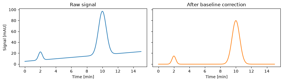
The threshold parameter selects baseline points by normalized intensity: only points whose normalized intensity falls below threshold (default 0.025, corresponding to the lowest 2.5 % of the signal range) are used for the linear fit. For broad peaks where few true baseline points are available, increase threshold. The optional start and end parameters restrict which points feed the fit, without zeroing or removing the rest of the signal. In practice this is useful when an artifact in part of the run (such as the ghost peak above) would otherwise bias the baseline estimate; the fitted line is then extrapolated across the full signal.

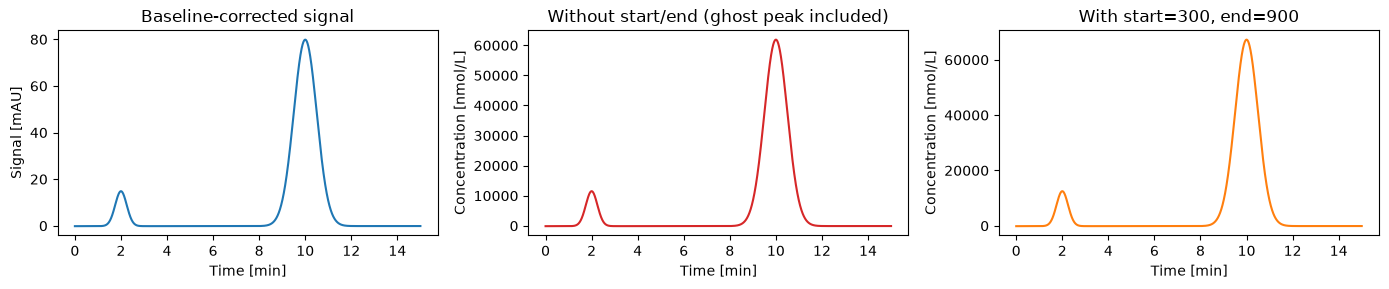
Area normalization

When the injected amount of a component is known exactly, normalize_area() rescales the signal so that the flow-weighted time integral matches the known injected amount (e.g. in mol or kg). This avoids the need for a calibration curve when the injection amount is precisely controlled. For multi-component mixtures or when extinction coefficients are available, Beer-Lambert or polynomial calibration is more appropriate.

The start and end parameters restrict the integration window. Without them, any artifact in the signal (such as the ghost peak carried over from baseline correction) is included in the integral, inflating the estimated amount and producing a wrong scale factor.

injected_mass = 5e-9  # mol

normalized = normalize_area(corrected, target_area=injected_mass,
                            start=300, end=900)
normalized_wrong = normalize_area(corrected, target_area=injected_mass)

correct_baseline_and_normalize() chains baseline correction and area normalization in one call for the common case where both steps are needed.

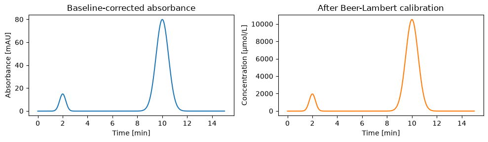
Beer-Lambert calibration

Beer-Lambert calibration converts UV absorbance signals (typically measured in AU or mAU) to concentration using a known molar extinction coefficient, without running standards. The relation \(A = \varepsilon \cdot c \cdot l\) gives \(c = A / (\varepsilon l)\), where \(\varepsilon\) is the molar extinction coefficient in L/(mol·cm) and \(l\) is the optical path length in cm.

# Extinction coefficient for lysozyme at 280 nm
epsilon = 38_000  # L / (mol·cm)
path_length = 0.2  # cm, typical for analytical UV cells

concentration = apply_beer_lambert(corrected, epsilon, path_length)

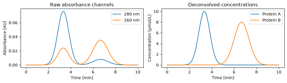
Multi-wavelength deconvolution

When several components absorb at the same wavelength, a single UV channel cannot separate their contributions. deconvolve_extinction() recovers per-component concentration profiles by solving the linear system

\[A_\lambda(t) = l \sum_i \varepsilon_{i,\lambda} \, c_i(t)\]

simultaneously across all wavelength channels, where \(\varepsilon_{i,\lambda}\) is the molar extinction coefficient of component \(i\) at wavelength \(\lambda\). These coefficients are assembled into an extinction matrix \(E \in \mathbb{R}^{n_\lambda \times n_\text{comp}}\), with rows corresponding to wavelengths and columns to components. The system is solved in the least-squares sense; using more wavelengths than components (\(n_\lambda > n_\text{comp}\)) improves robustness to measurement noise.

time_dec = np.linspace(0, 600, 6001)

# Extinction matrix: rows = wavelengths (280, 260 nm), columns = components (A, B)
E = np.array([
    [38_000, 5_000],   # ε at 280 nm
    [12_000, 22_000],  # ε at 260 nm
])
path_length = 0.2  # cm

# Simulate two overlapping peaks from known concentrations
c_A = 1e-5 * np.exp(-0.5 * ((time_dec - 200) / 30) ** 2)
c_B = 8e-6 * np.exp(-0.5 * ((time_dec - 400) / 40) ** 2)
A_mat = np.stack([c_A, c_B], axis=1) @ E.T * path_length
ref_280 = ReferenceIO("A280", time_dec, A_mat[:, 0:1], flow_rate=1e-6)
ref_260 = ReferenceIO("A260", time_dec, A_mat[:, 1:2], flow_rate=1e-6)

results = deconvolve_extinction(
    [ref_280, ref_260], E, path_length,
    component_names=["Protein A", "Protein B"],
)

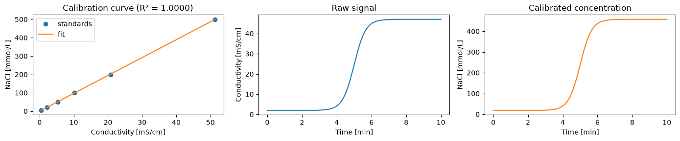
Polynomial calibration from standards

For detectors where Beer-Lambert does not apply, such as conductivity detectors, fit_polynomial() fits a calibration curve from (signal, concentration) standard measurements and returns the polynomial coefficients together with \(R^2\).

# Standard measurements: conductivity vs. NaCl concentration
conductivity_standards = np.array([0.5, 2.1, 5.3, 10.2, 20.8, 51.3])  # mS/cm
nacl_concentration = np.array([5, 20, 50, 100, 200, 500])  # mmol/L

coeffs, r2 = fit_polynomial(conductivity_standards, nacl_concentration, degree=1)
print(f"R² = {r2:.4f}")

time_cond = np.linspace(0, 600, 6001)
conductivity = (2 + 45 * (1 / (1 + np.exp(-0.05 * (time_cond - 300))))).reshape(-1, 1)
ref_cond = ReferenceIO("Conductivity", time_cond, conductivity, flow_rate=1e-6)

ref_nacl = apply_polynomial_calibration(ref_cond, coeffs)

R² = 1.0000