The Yamamoto method

The Yamamoto method [13] estimates the two key SMA binding parameters, characteristic charge \(\nu\) and equilibrium constant K, from a small set of linear salt-gradient elution (LGE) experiments, without requiring an inverse problem to be solved.

Theory

For a protein eluting under a linear salt gradient, the normalized gradient slope \(GH\) and the peak salt concentration \(I_R\) are related by [14]:

\[ \log(GH) = (\nu + 1)\,\log(I_R) - \log\!\bigl(K \cdot \Lambda^\nu \cdot (\nu + 1)\bigr) \]

where \(\Lambda\) is the resin ionic capacity (mM, per solid-phase volume) and concentrations are in M. \(GH\) is computed from the gradient slope and the column void volume:

\[ GH = \frac{c_{\mathrm{salt,end}} - c_{\mathrm{salt,start}}}{V_{\mathrm{gradient}}} \cdot V_{\mathrm{solid}} \]

with \(V_{\mathrm{solid}} = (1 - \varepsilon_t)\,V_{\mathrm{column}}\).

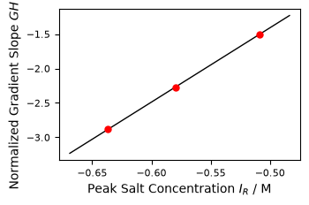
Running the same experiment at several gradient lengths (i.e. different \(GH\) values) produces a straight line in \(\log GH\) vs \(\log I_R\) space. A linear regression then yields:

• slope \(\rightarrow\) \(\nu + 1\), so \(\nu\) is recovered from the slope

• intercept \(\rightarrow\) \(K\)

Setup requirements

The linear gradient must start at the same salt concentration as the column equilibration buffer. A salt step-up before the ramp can partially desorb weakly-retained proteins, causing incorrect parameter estimates even when R² remains high.

\(\nu\) is recovered from the slope of the log-log plot and is generally robust. \(K\) is recovered from the intercept and is more sensitive to band-broadening: columns with more theoretical plates (\(N = u_{\mathrm{inter}} L / 2 D_{\mathrm{ax}}\)) give more accurate \(K\) estimates.

Example

import numpy as np

from CADETProcess.processModel import ComponentSystem
from CADETProcess.tools.yamamoto import GradientExperiment, fit_parameters

from binding_model_parameters import create_column_model, create_in_silico_experimental_data

if __name__ == "__main__":
    component_system = ComponentSystem(['Salt', 'Protein'])
    column = create_column_model(component_system, final_salt_concentration=600, initial_salt_concentration=50)

    column_volume = column.length * ((column.diameter / 2) ** 2) * np.pi

    create_in_silico_experimental_data()

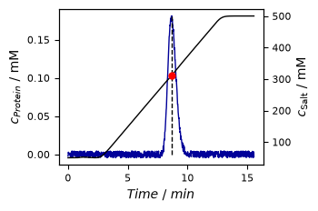
    exp_5cv = np.loadtxt("experimental_data/5.csv", delimiter=",")
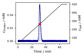
    exp_30cv = np.loadtxt("experimental_data/30.csv", delimiter=",")
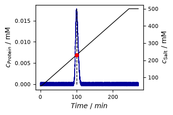
    exp_120cv = np.loadtxt("experimental_data/120.csv", delimiter=",")

    experiment_1 = GradientExperiment(exp_5cv[:, 0], exp_5cv[:, 1], exp_5cv[:, 2], 5 * column_volume)
    experiment_2 = GradientExperiment(exp_30cv[:, 0], exp_30cv[:, 1], exp_30cv[:, 2], 30 * column_volume)
    experiment_3 = GradientExperiment(exp_120cv[:, 0], exp_120cv[:, 1], exp_120cv[:, 2], 120 * column_volume)

    experiments = [experiment_1, experiment_2, experiment_3]

    for experiment in experiments:
        experiment.plot()

    yamamoto_results = fit_parameters(experiments, column)

    print('yamamoto_results.characteristic_charge =', yamamoto_results.characteristic_charge)
    print('yamamoto_results.k_eq =', yamamoto_results.k_eq)

    yamamoto_results.plot()

yamamoto_results.characteristic_charge = [9.7878889]
yamamoto_results.k_eq = [0.0753743]